Choose where make-to-stock ends and make-to-order begins

Why single-mode planning fails multi-variant factories

Most industrial equipment, valve, motor and pump manufacturers do not run a pure Make-to-Stock (MTS) or pure Make-to-Order (MTO) plant. Their catalogue contains a few dozen high-volume standard items that distributors expect within 48 hours, hundreds of modular configurations with interchangeable motors, seals and flange drillings, and a long tail of special alloy or custom skid builds.

When planners apply a single ERP planning strategy across that entire spectrum, two failure loops appear:

1. The MTS inventory trap: Holding finished-goods safety stock across hundreds of low-volume variants ties up working capital in slow-moving combinations while standard runners still stock out because assembly capacity was consumed building speculative variants.
2. The MTO whip-saw: Treating every order as custom make-to-order floods the machine shop with small-lot setups, stretches standard lead times beyond market tolerance and causes sales teams to mark orders urgent—cannibalizing common components needed for routine replenishment.

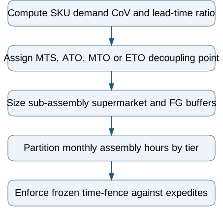
Choose where make-to-stock ends and make-to-order begins — reporting workflow

Follow the workflow below, or open its complete text version.

Read the complete workflow as text

1. Compute SKU demand CoV and lead-time ratio → Assign MTS, ATO, MTO or ETO decoupling point
2. Assign MTS, ATO, MTO or ETO decoupling point → Size sub-assembly supermarket and FG buffers
3. Size sub-assembly supermarket and FG buffers → Partition monthly assembly hours by tier
4. Partition monthly assembly hours by tier → Enforce frozen time-fence against expedites

Quantitative rules for positioning the decoupling point (CODP)

The Customer Order Decoupling Point (CODP) is the exact level in the Bill of Materials where forecast-driven push stock ends and customer-order-driven pull execution begins. Planners can classify each SKU into one of four policies using two coordinates:

• Demand Variability (CoV): Weekly standard deviation of demand divided by mean weekly demand (σ ÷ μ).
• Lead-Time Ratio (LTR): Customer-accepted delivery lead time divided by total cumulative manufacturing and procurement lead time (LT_customer ÷ LT_cumulative).

1. Make-to-Stock (MTS) — CoV up to 0.35 and LTR below 0.25

High-runner standard configurations where customers expect immediate dispatch (2 days) against an 18-day manufacturing cycle. The decoupling point sits at the Finished Goods Warehouse (FG-WH), replenished via min/max or Kanban loops.

2. Assemble-to-Order (ATO) — CoV 0.36 to 0.80 and LTR 0.25 to 0.50

Modular families where common machined casings, shafts, impellers and motor frames combine into dozens of end-item permutations. The decoupling point sits at the Machined Sub-Assembly Supermarket (WIP-SUPERMARKET). Sub-assemblies are machined to forecast; final assembly, painting and hydro-testing trigger only when a customer order arrives (7-day promised lead time versus 24-day cumulative cycle).

3. Make-to-Order (MTO) — CoV 0.81 to 1.80 and LTR 0.50 to 1.00

Special alloy variants or non-standard flange drillings where customers accept a 21-day lead time. The decoupling point sits at Raw Castings and Bar Stock (RAW-STORE). No machining or assembly starts without a confirmed sales order.

4. Engineer-to-Order (ETO) — CoV above 1.80 and LTR above 1.00

Custom engineered skids where unique design and long-lead procurement start after order confirmation (45–60 days). Only common fasteners and instrumentation sit in buffer stock.

Worked example: 320-SKU centrifugal pump plant (PLANT-PMP-02)

Consider illustrative industrial pump plant PLANT-PMP-02, which manages 320 active SKUs, ships 2,500 pumps per month and operates 1,200 monthly assembly and hydro-test hours. To prevent MTO expedites from starving standard distributor replenishment, the Master Production Schedule partitions both strategic inventory buffers and monthly capacity across the four decoupling tiers:

Why hybrid decoupling outperforms pure MTS or pure MTO

1. ₹48,00,000 working-capital reduction via ATO: Stocking finished goods for all 110 modular stainless pump variants to support a 7-day lead time would require ₹1,04,00,000 in finished stock. Holding the buffer one level lower in shared wet-ends, shafts and motors requires ₹56,00,000 (₹48,00,000 lower capital tied up) while meeting the 7-day assembly window.
2. Protected capacity lanes: Reserving 540 hours (45.00%) for MTS replenishment, 360 hours (30.00%) for ATO final assembly, 210 hours (17.50%) for MTO orders and 90 hours (7.50%) for ETO skids ensures that a surge in custom MTO bookings extends only the MTO Available-to-Promise (ATP) queue rather than draining MTS distributor stock.

Implementation checklist for hybrid MPS/MRP

• BOM decoupling flags: Set planning_method = MTS | ATO | MTO | ETO at both the parent SKU and sub-assembly BOM levels so MRP stops exploding forecast demand below the decoupling buffer.
• Frozen time fence (0–5 days): Lock the assembly schedule inside a 5-day frozen window where MTO expedites cannot displace scheduled MTS replenishment without plant manager approval.
• Quarterly CoV review: Recompute rolling 26-week CoV every quarter to promote stabilized MTO items into ATO and demote volatile MTS items back to ATO or MTO.